PDE Example: Diffusion in a box (Same as heat)
We look the time-evolution of the distribution of small particles as they spread due to diffusion, but are confined to a 1D box. The box has length L.
The Diffusion equation is:
Contents

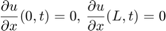
Boundary conditions for the closed box case are:
We can see that the following is a solution to the differential equation:
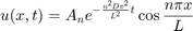
where  are determined by the intial distribution
  .
.
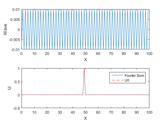
%Setup problem and initial state
L=100;          %Length of box
D=1;            %Diffusion Constant
U0=zeros(1,L);  %This is our t=0 particle distribution u(x,0)
U0(50)=1;       %Make this a delta function (we dropped a small drop of ink into the middle of 1D glass of water)

X=(0:L-1);
N=length(X)

%Calculate the Coefficients
A0=1/L*sum(U0);
for nn=1:N-1
    An(nn)=2/L*sum(U0.*cos(nn*pi*X/L));
end
An(N)=1/L*sum(U0.*cos(N*pi*X/L));
%Note the special end cases.  This correction is required to to exactly represent the U0 using an
%orthognal set of cosine base functions. The term An(N) is different in the
%discrete sampling case.

% Calculates a term in the series sum.
DiffEq = @(A,t,n,x)A*exp(-(n^2*D*pi^2*t/L^2))*cos(n*pi*x/L);

%Show the series sum to represent U0
X=(0:L-1);
t=0;
U=A0;
figure
for nn=1:N
    Wave=DiffEq(An(nn),t,nn,X);
    U=U+DiffEq(An(nn),t,nn,X);
    subplot(2,1,1);
    plot(X,Wave)
    xlabel('X');ylabel('Wave')
    subplot(2,1,2);
    hold off
    plot(X,U)
    hold on;
    plot(X,U0,'r--');
    xlabel('X');ylabel('U')
    %pause(.01)
end
legend('Fourier Sum','U0')
N =

   100
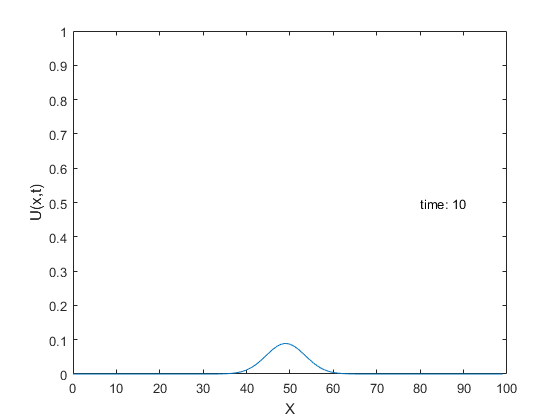
Show the time evolution:
We simply evaluate the series at different time points.
figure
for tt=0:.1:10
    U=A0;
    for nn=1:N
        U=U+DiffEq(An(nn),tt,nn,X);
    end
    plot(X,U)
    xlabel('X');ylabel('U(x,t)')
    s=sprintf('time: %g',tt);
    text(80,.5,s);
    axis([0 L 0 1])
    %pause(1)
end